Visualizing convolutional neural networks outputs
Convolutional neural networks (CNNs) are the type of neural networks the more likely to allow us to understand what is happening internally, since, as opposite to many other type of neural nets (I am thinking to GANs for example), CNNs are basically a representation of visual concepts.
Either for the purpose of debugging, or the personal satisfaction of visualizing the magic happening in your neural network, visualizing the network interpretations of your input is absolutely necessary to master when getting into deep learning. I will start by interpreting the most helpful method I discovered : the heatmap visualization of class activations in the input image.
These posts are openly related to the “Deep learning with Keras” book. This is my interpretation of the content, in a way that would allow me to look back at it and understand the subject with my own words.
UPDATE : The pictures looks like they have just decided to disappear. I will do my best to find these demons and bring them back ASAP.
UPDATE 2 : The pictures are all back and warned. They won’t run away again any soon.
Convolutional neural networks (CNNs) are the type of neural networks the more likely to allow us to understand what is happening internally, since, as opposite to many other type of neural nets (I am thinking to GANs for example), CNNs are basically a representation of visual concepts.
Either for the purpose of debugging, or the personal satisfaction of visualizing the magic happening in your neural network, visualizing the network interpretations of your input is absolutely necessary to master when getting into deep learning. I will start by interpreting the most helpful method I discovered : the heatmap visualization of class activations in the input image. Let’s refer to it as HVCA.
The idea behind HVCA
HCVA basically represents which part of the input image led to the activation of a specific class. In other words, it allows you to visualize what object or entity in the image the network has been able to interpret, thus leading him to this decision.
The HCVA is part of a category of visualization techniques called CAM, which is short for class activation map.The idea is to obtain a matrix of values representing the score of a specific output class (for example, the car class if a car is displayed in the image), for every single location of the image. This matrix indicate how important each location in the input image have been to lead to the activation of the class.You can produce a heatmap for every single class of your classifier, ranging from the most activated to the less activated.
You will probably see similar areas activating multiple classes, which is normal and depending of the layer you chose to produce your heatmap on. Bottom layers tend to encode relatively simple and general features, so your heatmap will be roughly the same for every class you decide to base it on. But as you get further in the network, you will start seeing specific parts of the image being highlighted by the heatmap.The HCVA implementation described on the book is itself based on the “Grad-CAM: Visual Explanations from Deep Networks via Gradient-based Localization.” paper.
The idea behind is quite simple for maths lovers, less simple for others. Quite frankly, if you managed to understand how CNNs work and the theory behind, this one should be easy to grasp.
The idea is to weigh every channel in the feature map resulting from a convolutional layer by the gradient of the class with respect to the channel. We can divide this process by four main steps :
- We first need to feed the image to the network
- We need to get the output feature map of the layer we want our heatmap to be based on
- We need to compute the gradient of the class with regards to the output feature map we previously got
- Finally, we multiply every channel of the feature map by the computed gradient for each channel
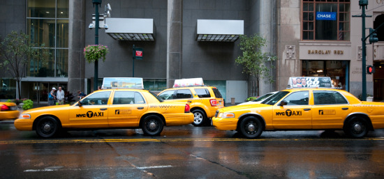
We will be using the VGG16 model, since it comes already packaged with keras, and the library also provides many utilities functions to simplify our task.Let’s pick an image from the internet, displaying some new york cabs, that the network is bound to classify :
I first load the vgg16 full model, then preprocess the image, such as resizing it to fit the 226x226 format that the model accepts, convert it into a Numpy float32 tensor and apply some more preprocessing rules.
Why do we do this ? Basically because a JPG or PNG image is made of multiple layers, that plays on the compression of the picture, and many more parameters, that would take a whole article to describe.
    from keras.applications.vgg16 import VGG16, preprocess_input, decode_predictions
    from keras.preprocessing import image
    import numpy as np

    def preprocess_image(img_path):
        img = image.load_img(img_path, target_size=(224, 224))
        x = image.img_to_array(img)
        x = np.expand_dims(x, axis=0) #Insert a new axis to alter the shape of x
        x = preprocess_input(x) #Will scale pixels between -1 or 1 to avoid erratic behavior
        return x
Let’s run the model on our picture now :
       if __name__ == ' __main__':
           model = VGG16(weights='imagenet')
           img_path = \"/home/mehanna/Documents/Programming/hcvavgg/nyc-taxi.jpg\"
           preds = model.predict(preprocess_image(img_path))
           print(\"Predicted:\", decode_predictions(preds, top=2)[0])
Which results in :
> Predicted: [('n02930766', 'cab', 0.994823), ('n04146614', 'school_bus', 0.0026146742)]
We can see that the top three classes predicted are :
- Cab with 99.5% probability
- School bus with 0.26% probability
Our network is working as expected as it has recognized the cab as mainly displayed in the picture, so the corresponding class was maximally activated. Let’s find out the index of the cab in the prediction vector :
    np.argmax(preds[0])
    > 468
Now let’s try to visualize which part of the image led the network to this prediction, by setting up the Grad-CAM algorithm. First, let’s visualize the model :
:
    >>>model.summary()
        _________________________________________________________________
        Layer (type)                 Output Shape              Param #
        =================================================================
        input_1 (InputLayer)         (None, 224, 224, 3)       0
        _________________________________________________________________
        block1_conv1 (Conv2D)        (None, 224, 224, 64)      1792
        _________________________________________________________________
        block1_conv2 (Conv2D)        (None, 224, 224, 64)      36928
        _________________________________________________________________
        block1_pool (MaxPooling2D)   (None, 112, 112, 64)      0
        _________________________________________________________________
        block2_conv1 (Conv2D)        (None, 112, 112, 128)     73856
        _________________________________________________________________
        block2_conv2 (Conv2D)        (None, 112, 112, 128)     147584
        _________________________________________________________________
        block2_pool (MaxPooling2D)   (None, 56, 56, 128)       0
        _________________________________________________________________
        block3_conv1 (Conv2D)        (None, 56, 56, 256)       295168
        _________________________________________________________________
        block3_conv2 (Conv2D)        (None, 56, 56, 256)       590080
        _________________________________________________________________
        block3_conv3 (Conv2D)        (None, 56, 56, 256)       590080
        _________________________________________________________________
        block3_pool (MaxPooling2D)   (None, 28, 28, 256)       0
        _________________________________________________________________
        block4_conv1 (Conv2D)        (None, 28, 28, 512)       1180160
        _________________________________________________________________
        block4_conv2 (Conv2D)        (None, 28, 28, 512)       2359808
        _________________________________________________________________
        block4_conv3 (Conv2D)        (None, 28, 28, 512)       2359808
        _________________________________________________________________
        block4_pool (MaxPooling2D)   (None, 14, 14, 512)       0
        _________________________________________________________________
        block5_conv1 (Conv2D)        (None, 14, 14, 512)       2359808
        _________________________________________________________________
        block5_conv2 (Conv2D)        (None, 14, 14, 512)       2359808
        _________________________________________________________________
        block5_conv3 (Conv2D)        (None, 14, 14, 512)       2359808
        _________________________________________________________________
        block5_pool (MaxPooling2D)   (None, 7, 7, 512)         0
        _________________________________________________________________
        flatten (Flatten)            (None, 25088)             0
        _________________________________________________________________
        fc1 (Dense)                  (None, 4096)              102764544
        _________________________________________________________________
        fc2 (Dense)                  (None, 4096)              16781312
        _________________________________________________________________
        predictions (Dense)          (None, 1000)              4097000
        =================================================================
        Total params: 138,357,544
        Trainable params: 138,357,544
        Non-trainable params: 0
We will focus on visualizing what in the last conv layer, led to the activation of the cab class.
    from keras import backend as K
    import matplotlib.pyplot as plt

    def grad_cam(model, x):
        cab_output = model.output[:, 468]
        last_conv_layer = model.get_layer('block5_conv3')
        grads = K.gradients(cab_output, last_conv_layer.output)[0] #Gradient in respect to the cab entries
        pooled_grads = K.mean(grads, axis=(0, 1, 2))
        iterate = K.function([model.input], [pooled_grads, last_conv_layer.output[0]])
        pooled_grads_value, conv_layer_output_value = iterate([x])
        for i in range(512): #We basically execute the previously described algorithm
            conv_layer_output_value[:, :, i] *= pooled_grads_value[i]
       #Building the heatmap, channel wise mean
       heatmap = np.mean(conv_layer_output_value, axis=-1)
       #Standarizing the values between 0 and 1
       heatmap = np.maximum(heatmap, 0)
       heatmap /= np.max(heatmap)
       plt.matshow(heatmap)
       plt.show()
I had a hard time understanding the point of the keras.backend.function, this Stackoverflow answer does a great job explaining.It is basically a simple mapping from an input to an output.
The displayed heatmap looks like this for me :

We can clearly see that the rightmost cab is the one that mostly triggered the network and led to the prediction. Let’s superpose the heatmap to our original picture :
    import cv2

    def generate_heatmap_on_image(img_path, heatmap):
        img = cv2.imread(img_path)
        heatmap2 = np.copy(heatmap)
        heatmap2 = cv2.resize(heatmap2, (img.shape[1], img.shape[0]))
        heatmap2 = np.uint8(255 * heatmap2)
        heatmap2 = cv2.applyColorMap(heatmap2, cv2.COLORMAP_JET)
        final_image = heatmap2 * 0.4 + img
        cv2.imwrite('/home/mehanna/Documents/Programming/hcvavgg/cab_cam.jpg', final_image)
The resulting picture is pretty straightforward to understand :
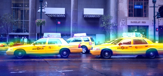
Quite surprisingly, the windows mostly triggered the model, along with the little sign, which I imagined would have been the main reason the network output the cab prediction.
Conclusion
The heatmap visualisation is an extremely powerful technique to debug our network if we feel the prediction are not accurate, or far from expected. It is very easy to implement using keras. Other methods will be discussed but this one is definitely a must if we need to debug a convnet.
The “Deep learning with keras” book does a great job explaining in more details than I did. I basically interpreted their words in order to make it easier for me to understand in the future.
Full code :
    from keras.applications.vgg16 import VGG16, preprocess_input, decode_predictions
    from keras.preprocessing import image
    from keras import backend as K
    import matplotlib.pyplot as plt
    import numpy as np
    import cv2

    def preprocess_image(img_path):
        img = image.load_img(img_path, target_size=(224, 224))
        x = image.img_to_array(img)
        x = np.expand_dims(x, axis=0) #Insert a new axis to alter the shape of x
        x = preprocess_input(x)
        #Will scale pixels between -1 or 1 to avoid erratic behavior
        return x

    def grad_cam(model, x):
        cab_output = model.output[:, 468]
        last_conv_layer = model.get_layer('block5_conv3')
        grads = K.gradients(cab_output, last_conv_layer.output)[0] #Gradient in respect to the cab entries
        pooled_grads = K.mean(grads, axis=(0, 1, 2))
        iterate = K.function([model.input], [pooled_grads, last_conv_layer.output[0]])
        pooled_grads_value, conv_layer_output_value = iterate([x])
        for i in range(512): #We basically execute the previously described algorithm
            conv_layer_output_value[:, :, i] *= pooled_grads_value[i]
        #Building the heatmap, channel wise mean
        heatmap = np.mean(conv_layer_output_value, axis=-1)
        #Standarizing the values between 0 and 1
        heatmap = np.maximum(heatmap, 0)
        heatmap /= np.max(heatmap)
        plt.matshow(heatmap)
        #plt.show()

        return heatmap

     def generate_heatmap_on_image(img_path, heatmap):
         img = cv2.imread(img_path)
         heatmap2 = np.copy(heatmap)
         heatmap2 = cv2.resize(heatmap2, (img.shape[1], img.shape[0])
         heatmap2 = np.uint8(255 * heatmap2)
         heatmap2 = cv2.applyColorMap(heatmap2, cv2.COLORMAP_JET)
         final_image = heatmap2 * 0.4 + img
         cv2.imwrite('/home/mehanna/Documents/Programming/hcvavgg/cab_cam.jpg', final_image)

     if __name__ == ' __main__':
         model = VGG16(weights='imagenet')
         model.summary()
         img_path = "/home/mehanna/Documents/Programming/hcvavgg/nyc-taxi.jpg"
         x = preprocess_image(img_path)
         preds = model.predict(x)
         print(\"Predicted:\", decode_predictions(preds, top=3)[0])
         print(np.argmax(preds[0]))
         heatmap = grad_cam(model, x)
         generate_heatmap_on_image(img_path, heatmap)