Efficiently working with Spark partitions

It’s been quite some time since my last article, but here is the second one of the Apache Spark serie. For those of you that are new to spark, please refer to the first part of my previous article which introduces the framework and its usages. In this article, I will show how to execute specific code on different partitions of your dataset. The use cases are various as it can be used to fit multiple different ML models on different subsets of data, or generate features that are group-specific, and more.
It’s been quite some time since my last article, but here is the second one of the Apache Spark serie. For those of you that are new to spark, please refer to the first part of my previous article which introduces the framework and its usages. In this article, I will show how to execute specific code on different partitions of your dataset. The use cases are various as it can be used to fit multiple different ML models on different subsets of data, or generate features that are group-specific, and more.
Spark parallelism
In this section, we aim to review how Spark is able to perform parallel operations on your dataset. For this purpose, we will first discuss how Spark represents your data and how this representation allows the framework to make the most of parallel computation. We will then review how Spark makes us of your cluster to distribute the data and perform actions on it. Finally, we will briefly go through how Spark organizes your actions and present some guidelines for avoiding OOMs and speed up your code.
Data abstractions
Currently, Apache Spark offers three data abstractions, each with its set of pros and cons:
- RDDs: RDDs have been the main data abstraction on Spark since its release. It stands for Resilient Distributed Dataset. Behind these words hides the definition of what makes RDDs special: it is a resilient, partitioned, distributed and immutable collection of data.
- Resilient means that RDDs are able to recover quickly of a failure. This aspect is enforced by the immutability of the data structure (see below).
- Immutable means that once an RDD is defined, it cannot be modified. Every action on an RDDs yields another RDD. This aspect helps RDDs be more resilient, since if one operation fails, it can revert to the previous created RDDs (to some extent).
- Partitioned: Spark partitions your data into multiple little groups called partitions which are then distributed accross your cluster’s node. This enables parallelism.
- RDDs are a collection of data: quite obvious, but it is important to point that RDDs can represent any Java object that is serializable.
- Dataframe: the dataframe is based upon RDDs and has been introduced a bit later than RDDs, in Spark 1.3, with the purpose to serve for the Spark SQL module. Dataframes are organized into named columns and are quite close to Panda’s dataframes. Spark recommends the use of dataframes for development, but it should be noted that they offer a higher level of abstraction than RDDs and thus, their range of action is less broad. Dataframes, in the context of Spark SQL allow you to perform SQL like queries in order to play on your data.
- Datasets: they were the latest introduction of Spark, making their grand entering in Spark 1.6. Datasets combine both the advantages of Dataframes and RDDs as one can run SQL like queries on them and also perform functional operations such as mapPartitions (which we will review later).
So among these three data abstractions, which one should you use ?
Well it really depends on the level of control you want and the goal you want to achieve. Datasets are regularly a good choice to go with as it allows you to read and parallelize data the same way as RDDs and still want a structured (or semi-structured) representation of your data as Spark automatically infers your data’s representation. Plus, as we see next, Datasets emphasize both RDDs and Dataframes. For instance, a Dataframe is basically only a Dataset[Row]
Dataframes should be used if you need a high level of abstraction on your data and don’t want to mess too much with the optimization: Dataframes come with two powerful optimizers named Catalyst and Tungsten. Catalyst for instance takes your code and generates optimized physical and logical query plans. These optimizers delete by themselves useless queries, combine queries that can be executed together, etc… Going deep into these optimizers would be moving away from the subject.
Finally, I personally use RDDs only when I cannot perform my actions using Datasets or Dataframes. RDDs don’t have any optimizers to my knowledge, and can be a hassle managing as they suffer a lot of GC (Garbage Collection) issues (these issues are known to impact Datasets as well, but in a lesser way).
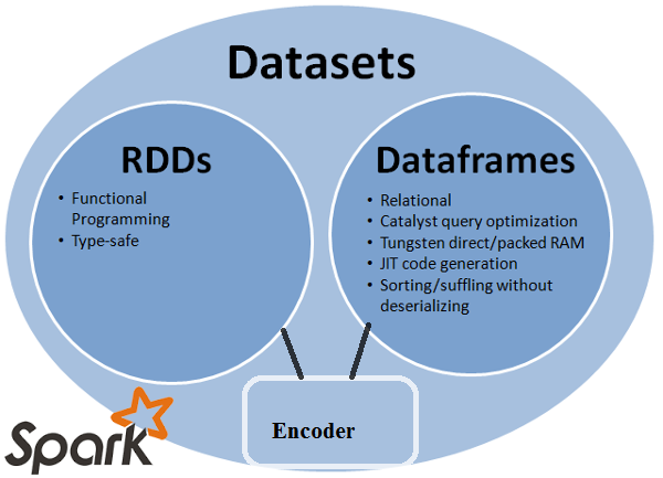
The previous picture summarizes how these three data abstractions relate to each others. Note how the Dataset seems to encapsulate both the advantages of RDDs and Dataframes. However, it also encapsulates most of their disadvantages. You can also note the reference to “encoders”: the Dataset API has this concept of encoders which can translate between JVM representations towards Spark’s internal binary format. (see this SO thread for improved details)
Spark jobs
In this section we will rapidly review how Spark constructs its job processes and how they are effectively executed. Once Spark interprets and optimizes your code using Catalyst/Tungsten, containing multiple transformations leading to an action, it constructs a DAG, for Directed Acyclic Graph. This is the beginning of the Spark process.
DAGs (Directed Acyclic Graph)
The DAG is a graph that holds track of the operations applied to a RDD. It is a combination of edges and vertices that respectively indicate the operations and the RDDs. The DAG for each action can be seen in the SparkUI and looks this way :
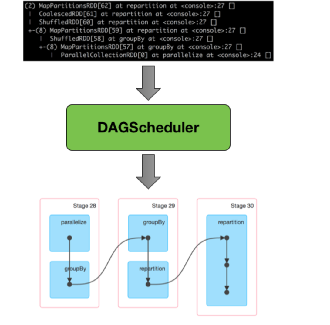
The DAG is an important scheduling layer in spark, as it converts the logical execution plan (generated by the Catalyst optimizer). The DAG is built following a series of lookup which (among many) separates the stages based on the transformation type:
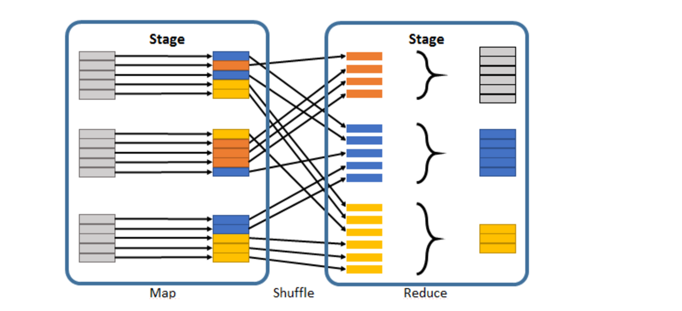
- A wide transformation involving a full shuffle of data accross partitions
- A narrow transformation performing map-side operations that do not require a shuffle of data.
Once the DAG has performed his lookups, it genereates the physical execution plan containing the different tasks.
Among its advantages, the DAG allows for a better fault-tolerance of your application as we can recover the lost RDDs by looking up the graph.
But wait, we mentioned stages and tasks, but concretely, what are these ?
Stages
Basically, one stage is a set of operation that does not involve a shuffle of data. As soon as a shuffle of data is needed, (when a wide transformation is performed), the DAG will yield a new stage.
Tasks
A task is generated for each action performed on a partition. We can only have as many tasks running in parallel as cores we have. That’s all we need to know about Spark tasks for now !
Spark partitions
Since we now know that Spark’s DataFrames and Datasets are both based on RDDs, our explanations will only focus on the latter.
What are partitions concretely ?
Partitions are chunks of your original (huge) dataset which are distributed over different nodes. Basically, RDDs are a collection of multiple partitions.
These partitions are quite easily customizable in number and in their constitution, as we will later see.
By default, when an HDFS file is read, Spark creates a logical partition for every 64 MB of data but this number can be easily modified by forcing it when parallelizing your objects or by repartitioning an existing RDD, by calling the .repartition() or .coalesce() methods.
The .repartition() leads to a full shuffle of data between the executors, leading to aggressive network traffic in order to divide the data into the specified number of partitions.
The .coalesce() operation is more optimized when it reduces the number of partitions, as it doesn’t trigger a full shuffle, but only a transfer of the data from partitions being removed to existing partitions.
Efficiently partitioning your data is important as a good partitioning can lead to huge speed improvement and fewer OOMs errors. This statement is even more true when your data is key-value oriented.
How does RDDs become key-value oriented ?
The key-value paradigm is essential in efficient parallel data processing. Spark provides full implementation of key-value based RDD in the PairRDD and the PairRDDFUnctions classes. These classes are made available through implicit conversion, meaning that you only have to create a regular RDD of a tuple (in scala), such as RDD[(key, value)], in order to be able to take advantages of its methods. Spark also provides the OrderedRDD and OrderedRDDFunctions classes for key-value oriented RDDs for which the key is ordered. (Note that the key must either have an implicit ordering defined, or you should define your implicit ordering function).
Needless to say that in order to exploit the full advantages of Spark parallelism, the partition must be created smartly, especially when we’re dealing with key-value RDDs.
The partitioning will define how most wide transformations scale up as they mostly are key-value transformations.
What are the considerations to have when dealing with key-value pairs ?
Dealing with key-value pairs should be well thought, before even starting to code as they can lead to numerous bottlenecks:
- The most frequent cause of OOMs errors comes from ineficient use of key-value partitioning, either on the driver, or on the executors. For instance, a .countByKey() operation on a huge number of keys may lead to OOMs exceptions on the driver, while actions performed on partition belonging to keys with too much entries may lead to OOMs on the executors.
- Bottlenecks tasks which slow down the whole job. They happen when the dataset is very unbalanced.
- Shuffle failure, which are caused by wide transformation weighing on the network traffic (shuffle read/write too high).
Can these problems be adressed through a good partitioning ?
Totally. Well, mostly. A smart partitioning can lead to less shuffle, and a smaller toll on the executor’s memory.
Also, a good architecture is essential in order to perform your actions in a smart way.
Having a good vision of your goal and a good knowledge of your data can help you build smart partitions. For instance, the keys should be no bigger than what can fit on the driver’s memory and the values per key should fit into the executor’s memory.
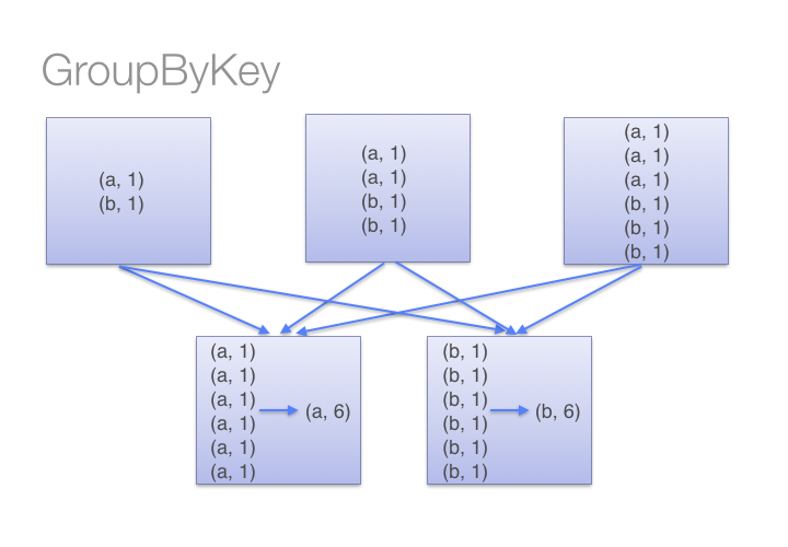
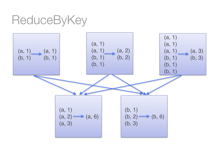
Extensive use of the .groupByKey() function is also not recommended as it leads to multiple OOMs errors if the partitioning is not built efficiently (or sometimes simply because your dataset has too many inputs). The .groupByKey() is essentially bad if one key has multiple duplicate values as it gather all the data for one key into one executor as an Iterator, which can rapidly explode in memory. Basically, you should avoid using functions that makes your accumulator bigger. For instance, functions such as .aggregateByKey() or reduceByKey() are implemented using map-side combinations, which means that they reduce the size of the accumulator for their partition, which makes them unlikely to yield OOMs exceptions.
For example, here is how groupByKey() versus reduceByKey() (performing a sum) behaves on data with many duplicates values:
How does Spark partition key-value pairs ?
Spark currently has two partitioners for your PairRDD (or OrderedRDD - remember, key-value pairs are implicitly converted from regular RDDs to PairRDDs or OrderedRDDs). One can call the .partitionBy() function on their key-value RDD to assign one of the two defined partitioners:
-
HashPartitioner: It is the default partitioner for pair RDDs in Spark (not ordered). It determines the index of a partition based on its hash value. The HashPartitioner takes a partition integer parameter to determine the number of partitions it will create. If this parameter is not specified, it is the spark.default.parallelism value that is used. (this parameter defaults to the number of all cores on your cluster). It is generally a good practice to define this parameter as you wish.
-
RangePartitioner: The range partitioner creates partitions with keys in the same range of defined values. This partitioner requires the keys to have an implicit ordering. The RangePartitioner takes, in addition to the number of partition, the parent PairRDD you want to sample.
Both RangePartitioner and HashPartitioner behave poorly on data with to many duplicates, possibly causing OOMs exceptions if the data for one key doesn’t fit in the executor memory.
Along with these two partitionners, it is also possible to define your CustomPartitioner in a quite straightforward way. To define a custom partitioner, you need to implement a series of mandatory and optional methods:
- Optional equals: a method to define equality between your partitioners.
- Optional hashcode: mandatory if the previous method has been defined.
- Mandatory numPartitions: returns the number of partitions as an integer.
- Mandatory getPartition: this method takes a key (of any given type you want to use) and returns its partition’s index.
We will defined one of our own custom partitioner in the next part so we can apply what we learned here.
There is a lot more to be said about partitioners but it would require a book to talk about everything. You should know that once your PairRDD is partitioned, it opens doors to multiple functions that act of these partitions (e.g .sampleByKey(), .mapPartitions(), etc…).
Use case: Performing alphabet/frequency sort on our dataset
Okay so the idea here is to work our way through RDDs and play with partitions. I thought that an easy way to use all the knowledge we gathered in the previous sections is to build a simple sorting tool.
I will walk through two versions: the first one is not very OOMs proof, and would not work with large and unbalanced datasets, while the other should adress this problem in a smarter way.
Version 1
So the idea here is to take an unsorted Dataframe with string columns, and sort string values for each key independently. We need to be able to achieve two type of sorting:
- Sorting by alphabet
- Sorting by frequency
Let’s go through the steps:
- Convert the dataframe to a PairRDD[(K, V)] with the value being the column we want to sort, and the key being the columns we partition by.
- Create our custom partitioner and partition our PairRDD with it so we can have one partition for each key.
- Write our .sortByAlphabet() and .sortByFrequency() functions.
- Map each partition and use either sortByAlphabet or sortByFrequency on them, and return an iterator with the the elements indexes.
For this purpose, let’s create a little mock dataset we will work with in this section:
// Importing spark implicits

import spark.implicits._

// Creating our mock dataset

val df = List(("a", "a"),
              ("a", "a"),
              ("a", "b"),
              ("a", "d"),
              ("b", "d"),
              ("b", "a")).toDF("key", "value")
Okay, let’s get started now !
We first need to create our PairRDD:
//Dataframes are basically a Dataset[Row] type, so mapping them makes us go through
//a Row object. I assume the columns are always Strings.

val myPairRDD = df.rdd.map(r => (r.getString(0), r.getString(1)))
Pretty easy, right ? We now need to create our custom partitioner. If you remember the previous section, we need to define only the .numPartitions() and .getPartition() methods:
import org.apache.spark.Partitioner

/*
We need to overrride the Partitioner class. Our partitioner take as a class constructor the list that will make the partition so it can derives the number and the index of partitions.
*/
class MyPartitioner(partitions: List[Any]) extends Partitioner {
    override val numPartitions: Int = partitions.length

    def getPartition(key: Any): Int = {
        val k = key.asInstanceOf[String]

        partitions.indexOf(k)
    }
}
That’s it. We just have to read the length of the used list to know the number of partitions, and we use that same list to return the index of the partition.
Let’s now write our sorting functions:
def sortByAlphabet(data: Seq[String],
                   ascending: Boolean,
                   key: Seq[String]): Array[(String, String, Int)] = {
    val sorted = data.filter(_ != null).sorted
    val sortedRes = if (ascending) {
        sorted.toArray
    } else {
        sorted.reverse.toArray
    }

    //We assum the key to be constant (as it's supposed to)
    (key.toArray, sortedRes, sortedRes.zipWithIndex.map(_._2)).zipped.toArray
}

def sortByFrequency(data: Seq[String],
                    ascending: Boolean,
                    key: Seq[String]): Array[(String, String, Int)] = {
    val freqs = data.groupBy(identity)
                     .mapValues(_.size)

    val sorted = data.map(s => (s, fresq(s)))
                     .sortBy(_._2)
                     .map(_._1)

    val sortedRes = if (ascending) {
        sorted.toArray
    } else {
        sorted.reverse.toArray
    }

    (key.toArray, sortedRes, sortedRes.zipWithIndex.map(_._2)).zipped.toArray
}
We have our two functions sorting our data. They are not the best sorting functions but they work, and that’s what we want for this first version. Now, let’s apply them to our partitions.
val listPartitions = data.select("key")
                         .distinct
                         .collect()

val data = myPairRDD.partitionBy(new MyPartitioner(listPartitions))
            .mapPartitions(iter => {
                val iterSeq = iter.toSeq
                sortByAlphabet(iterSeq.map(_._2), true, iterSeq.map(_._1)).toIterator
                // sortByFrequency(iterSeq.map(_._2), true, iterSeq.map(_._1)).toIterator
            })
In this code snippet, we repartition our data using our custom partitioner, and we map the partitions to apply our previous functions. The .mapPartitions() functions return an iterator that we convert to a sequence in order to read it multiple times. I decided to use the sortByAlphabet function here but it all depends on what we want.
Running this code works fine in our mock dataset, so we would assume the work is done. However, if we decide to run this code on a big dataset of a few thousand lines, this would undoubtedly fail. Why ?
Well, the partitions we constructed have been built in a bit of a stupid way. We learned nothing from the warnings of the previous sections: if one key has a lot of values, our repartitioning will lead to an OOM error since it wouldn’t fit on one iterator. This method would work if we are sure that our keys are well distributed and the iterators never go beyond the executor’s memory limit.
Is there a smarter way to do this ?
Yes, probably. And that is what we will try to do in the second version.
Version 2
Our first version was badly conceived, as it would often lead to OOM errors in producting on average datasets. But how can we make a better version ? Well, the good way to improve our code would be to simply let Spark handle the partitions, or partition in a smart way. We could set the number of partitions to approximately 3/4 times the number of available cores for instance as it would be just enough to let Spark handle the parallel operations efficiently without generating too much GC overhead. Our code would then be pretty separate depending on whether we want to perform a frequency sort, or an alphabet sort. Let’s review them:
- The common step would be to convert our dataframe to a more adapted representation. For both alphabet and frequency sorting, I decided to set as the key, a tuple of both the partitioning column and the value, and null as the value.
//Dataframes are basically a Dataset[Row] type, so mapping them makes us go through
//a Row object. I assume the columns are always Strings.

val myDataset: Dataset[(String, String)] = df.map(r => (r.getString(0), r.getString(1)))
val myKVDataset: Dataset[((String, String), Int)] = myDataset.map(r => ((r._1, r._2), null))
Alphabet sort:
- We can take advantage of scala’s implicits and simply call the .sortByKey() function. We would then use the implicit scala Tuple2 sort, which, by default, sort by the first value and then the second value of the tuple.
- We perform a narrow transformation and a partition sort to add a third column with the index. As we previously sorted by the key, we made sure that there would be no smaller value in the next partition. Once we have done so, we keep track of the maximum index for each of our partition keys in each physical partition.
- We map again through each partition and sum the sorting index with the maximum partition key in the previous logical partition.
val sortedDS: Dataset[(String, String)] = myKVDataset.sortByKey().map(k => (k._1, k._2))
We now have to gather the maximum index for each partition key.
val maxIndexes: Map[Int, Map[String, Int]] = sortedDS.mapPartitionsWithIndex((index, iter) => {
  val iterSeq = iter.toSeq
  Iterator((index, iterSeq.groupBy(_._1).map {
    case (key, value) => (key -> value.length)
  }))
}).collect().toMap
The .groupBy(_._1) return a list for each element of our grouping argument. It allows us to easily get the count of values for each key in each phyisical partition, that we gather as a Map mapping partition’s indexes to another map of key (from our partitioning column) and count.
Once we got our statistics, the only step left is to perform a map-side sort and sum the sorting index to the maximum index of the previous partition for our partition key. Note that if our previous Map is too heavy to fit in the executor’s memory, it will undoubtedly trigger an OOM error.
sortedRDD.map(r => (r._1._1, r._1._2)).mapPartitionsWithIndex((index, iter) => {
  val iterSeq = iter.toSeq
  val intermediateRes = iterSeq.groupBy(_._1).map {
    case (key, value) => value.zipWithIndex.map(r => (r._1._1, r._1._2, r._2))
  }.flatten

  if(index != 0)
    intermediateRes.map(k => (k._1, k._2, k._3 + maxIndexes.get(index-1).get.get(k._1).getOrElse(0))).toIterator
  else
    intermediateRes.map(k => (k._1, k._2, k._3)).toIterator
})
And we got our sorted dataset, without having to use a custom partitioner that would eventually explode in the executor’s memory. However, our method is not risk-free: by gather our statistics, we risk going beyond our executor’s limit and provoke a failure. We also use the .sortByKey() function. We also don’t take advantage of iterator-to-iterator transformations, as we convert our iterator to a regular sequence, causing the executor to read all the data at once, which, along with our statistic’s array, could explode in the memory.
Now for the frequency sort:
- We call the .countByKey() on our dataset. Note that if we have too much distinct keys here, this function will fail with an OOMs error on the driver. The .countByKey() function returns a map of key/count.
- We reformat our dataset to our original Dataset[(K, V)].
- Using this ordered map, we perform a map-side operation on the partition to assign the frequency for each key/value.
Let’s go through each step:
//Dataframes are basically a Dataset[Row] type, so mapping them makes us go through
//a Row object. I assume the columns are always Strings.

val myDataset: Dataset[(String, String)] = df.map(r => (r.getString(0), r.getString(1)))
val myKVDataset: Dataset[((String, String), Int)] = myDataset.map(r => ((r._1, r._2), null))
Mapping the row objects to a simple tuple allows us to get a Dataset[(String, String)]. We now have to call the .countByKey() operation:
val freqMap = myKVDataset.countByKey().toSeq
                .sortBy(_._2) //We get a Seq[((String, String), Long)]
                .map(k => (k._1._1, (k._1._2, k._2))) //Seq[(String, (String, Long))]
                .groupBy(_._1) //Map[String, ArrayBuffer[String, Long]]
                .map {
                    case (key, value) => (key -> value.map(r => r._2)
                                                      .zipWithIndex
                                                      .map(r => (r._1._1 -> r._2)).toMap))
                } //We get a Map[String, Map[String, Long]]
We now have Map with our partitions as keys and another Map as a value containing, for each value, its index in an ascending order. If we wanted the descending order, we could have simply added a .reverse (… -> .value.reverse).
We now define a little sorting function and use it on our original dataset:
def sortByFreq(data: Seq[(String, String)], freqMap: Map[String, Map[String, Int]]) = {
    data.map(s => (s._1, s._2, freqMap.get(s._1).get
                                      .get(s._2).getOrElse(0) + 1)) //Map's .get()   returns Options[Type]
}

val result = myDataset.mapPartitions(iter => {
    val iterSeq = iter.toSeq
    sortByFreq(iterSeq, freqMap).toIterator
})
That’s it. This sort will be performed by only two stages of limited impact. The biggest toll on ressources here is induced by the .countByKey() function. As we previously noted, too many distinct key/value pairs will cause the driver to fail. Note that our Map will also be distributed to our executors so if it explodes our executor’s memory, we may also face OOMs.
I tested both these sorts on a public dataset containing more than 2.3M rows, with many duplicate values and our version 2 managed to sort it in less than 15 seconds, while our version 1 failed to execute, as predicted on large datasets.
Conclusion
Spark is powerful when handling huge datasets and performing actions over these. We have seen that this performance is mostly due to how Spark handles your data with partitions, and how you should take into consideration all the Spark lifecycle and environment before writing your code. We have also seen how Spark perform operations on different partitions and how to design your code in such a way that it minimizes OOMs risks.
This is just a grasp on Spark’s power, and there is a lot more that can be done that we will review in future articles.
Sources
-
High Performance Spark: Best Practices for scaling and Optimizing Apache Spark (book) by Holden Karau/Rachel Warren